Description of Lorentz Transformations, the Doppler Effect, Hubble's Law, and Related Phenomena in Curvilinear Coordinates by Generalized Biquaternions

Alimzhan Kholmuratovich Babaev

doi:doi:10.11648/j.ajaa.20251201.12

Research Article |

| Peer-Reviewed

Description of Lorentz Transformations, the Doppler Effect, Hubble's Law, and Related Phenomena in Curvilinear Coordinates by Generalized Biquaternions

Alimzhan Kholmuratovich Babaev^*

Published in American Journal of Astronomy and Astrophysics (Volume 12, Issue 1)

Received: 11 December 2024 Accepted: 27 December 2024 Published: 22 January 2025

Views: Downloads:

Download PDF

Share This Article

Twitter
Linked In
Facebook

Abstract

This paper presents the derivation of Lorentz transformations in curvilinear coordinates utilizing generalized biquaternions. Generalized biquaternions are rotations in curvilinear coordinates, including on the tx, ty, and tz planes. These space-time rotations are precisely the Lorentz transformations in curvilinear coordinates. The orbital rotation of the source and/or receiver, which mathematically represents the Lorentz transformation in spherical coordinates, is identified as the cause of the transverse Doppler effect. The change in wave frequency, specifically the "redshift," results in nonlinearities of Hubble's law manifesting as phenomena such as accelerated and anisotropic expansion of the universe, aberration, and wave polarization. Apparently, redshift exists even without radial expansion of the universe, i.e., without the "Big Bang". The reasons for the accelerated expansion of the universe, the anisotropic (angular) distribution of relic radiation, and the polarization of light from distant stars become clear in this approach. This greatly simplifies the mathematical description and understanding of the supposedly complex processes occurring in the universe.

Published in	American Journal of Astronomy and Astrophysics (Volume 12, Issue 1)
DOI	10.11648/j.ajaa.20251201.12
Page(s)	9-20
Creative Commons	This is an Open Access article, distributed under the terms of the Creative Commons Attribution 4.0 International License (http://creativecommons.org/licenses/by/4.0/), which permits unrestricted use, distribution and reproduction in any medium or format, provided the original work is properly cited.
Copyright	Copyright © The Author(s), 2025. Published by Science Publishing Group

Keywords

Biquaternion, Lorentz Transformation, Redshift, Hubble's Law, Universe Expansion, Aberration, Starlight Polarization

1. Introduction

The cause of the wave frequency shift is attributed to the satellite's orbital motion, specifically the transverse motion of the signal source in a direction perpendicular to the observer. This phenomenon is known as the transverse Doppler effect

[1]

. The signal frequency offset (redshift) is a function of the orbital altitude and velocity of the satellite: Δω = f (h, v). Corrections

[2]

to adjust the data are consistently incorporated into the calculations in satellite navigation.

The classical formulation of the transverse Doppler effect (in the Cartesian coordinate system) represents a significant simplification that constrains the generalization of this principle to elucidate numerous phenomena.

The objective of this study is to derive the Lorentz transformation

[3]

and its associated phenomena, namely the Doppler effect and aberration, in a generalized form using curvilinear coordinates. This comprehensive approach offers universal applicability and facilitates a more profound understanding of various mechanisms, including the accelerated

[4]

and anisotropic

[5]

expansion of the Universe, as well as the nonlinear nature of the Hubble law and parameter

[6]

2. Results

2.1. Biquaternions in Cartesian Coordinates

In abstract (Clifford) algebra, rotations and transformations on planes in pseudo-Euclidean space are given by formulas:

x^{ʹ} = R_{α} x {\tilde{R}}_{α}

(1)

x = {\tilde{R}}_{α} x^{ʹ} R_{α}

(2)

Here R_α is a biquaternion, Ṝ_α is the inverse or complex-conjugate biquaternion

[7]

R_{α} ({\tilde{R}}_{α}) = I \cosh \frac{I η_{α} + γ φ_{α}}{2} \pm γ_{α} γ_{0} \sinh \frac{I η_{α} + γ φ_{α}}{2}

(3)

/orR_α(Ṝ_α) =exp(±γ_αγ₀z_α2)(4)

I is a unit 4 x 4 matrix; γ₀, γ_α (α =1, 2, 3) are Dirac matrices; γ = γ₀γ₁γ₂γ₃ is a matrix analog of the imaginary unit: γ² = - I; γ_αγ₀ z_α /2 is a bivector;

x = \sum_{i = 0}^{3} γ_{i} ∙ x^{i}

is the space-time vector in the stationary coordinate system (K);

x^{'} = \sum_{i = 0}^{3} γ_{i} ∙ x^{' i}

is the same vector in the moving coordinate system (K^’); z_α = I η_α + γ φ_α is a complex matrix.

φ_α are “purely spatial” rotations on the x0y, y0z, and z0x planes. Since we will only consider Lorentz transformations, we will omit these rotations in the following. η_α are angles of rotation of the t0x, t0y, and t0z planes, or so-called rapidities.

It is obvious that

R_αR_α^-1=R_αṜ_α=I(5)

The algorithm ((1) and/or (3)) is explained in various sources, such as

[8]

Note: If there is no sum sign (Σ_αx_α), then there is no summation, i.e., no summation over repeated indices (Einstein's summation). For example, there is no summation over α in R_α Ṝ_α or g_αα k^α x^α.

2.2. Biquaternions in Generalized Form

The generalization of the transformations (1) and (3) in curvilinear coordinates will be the following formulas:

x^{'} = R_{α} x {\tilde{R}}_{α}

(6)

x = {\tilde{R}}_{α} x^{'} R_{α}

(7)

Here

R_{α}

and

{\tilde{R}}_{α}

are a biquaternion and an inverse biquaternion in a generalized form

[9]

R_{α} ({\tilde{R}}_{α}) = \frac{1}{|τ_{α 0}|} (I |τ_{α 0}| \cosh \frac{z_{α}}{2} \pm τ_{α 0} \sinh \frac{z_{α}}{2})

(8)

x = \sum_{i = 0}^{3} e_{i} x^{i}

is a 4-vector in a fixed basis K;

x^{'} = \sum_{i = 0}^{3} e_{i} x^{' i}

is the same vector in the moving basis

K^{ʹ}

; τ_α0 = e_α ∧ e₀ is the bivector, i.e. the outer product of vectors e_α and e₀

[10]

;

|τ_α0 | = |e_α ∧ e₀ | = I(g_α0 g_α0-g₀₀ g_αα)^0.5is the modulus (“length”) of the bivector e_α ∧ e₀

[11]

; g_ij is a matric tensor; e_i are vectors in the system of curvilinear coordinates; ∧ and • are symbols of outer and inner products of vectors

[10]

The set of four such vectors {e_i} forms a local basis (frame) in the 4-dimensional space. It is obvious that the biquaternions (8) satisfy the condition:

R_{α} • {\tilde{R}}_{α} = I

Note. The name “vector” for e_i is conventional. In reality, e_i are 4 x 4 matrices related to Dirac matrices through coordinate transformation functions X_j (qⁱ):

e_{i} = \sum_{j = 0}^{3} \frac{\partial X_{j}}{\partial q^{i}} γ_{j}

2.3. Lorentz Transformation in Generalized Form

Let us find the explicit form of the transformation (7). Let us substitute the biquaternions xʹ and x (8) into (7).

According to Clifford's double cross product

[2]

z•(x∧y) =– (x∧y)•z= (z•x)y-(z•y)x(9),

we can write

x = {\tilde{R}}_{α} • x^{'} • R_{α} = {\tilde{R}}_{α} • {\tilde{R}}_{α} • x^{'}

(10)

Indeed, the identity

x^{'} • R_{α} = {\tilde{R}}_{α} • x^{'}

is the place to be, since vectors

e_{0} x^{' 0}

and

e_{α} x^{' α}

commutate with I(| e_α∧e₀|cosh(z_α/2) but anticommutate with I(e_α∧e₀)sinh(z_α/2).

In curvilinear coordinates, the products of

e_{0} • τ_{α 0}

and e₀•τ_α0 are

[12]

\{\begin{matrix} e_{0} • τ_{α 0} = e_{0} • (e_{α} \land e_{0}) = (e_{0} • e_{α}) e_{0} - (e_{0} • e_{0}) e_{α} = - g_{00} e_{α} \\ e_{α} • τ_{α 0} = e_{α} • (e_{α} \land e_{0}) = (e_{α} • e_{α}) e_{0} - (e_{α} • e_{0}) e_{α} = g_{αα} e_{0} \end{matrix}

(11)

For simplicity, we will consider an orthogonal coordinate system, i.e., e_i•e_j = g_ij, if i=j and e_i•e_j = 0, if i≠j. Accordingly |τ_α0 |= I(– g₀₀ g_αα)^0.5.

Then from equation (10) we get

e_{0} x^{0} + e_{α} x^{α} = \frac{I τ_{α 0}^{2} \cosh η_{α} + | τ_{α 0} | τ_{α 0} \sinh η_{α}}{τ_{α 0}^{2}} • (e_{0} x^{' 0} + e_{α} x^{' α})

We substitute (11.1) and (11.2) into this equality. Multiplying the brackets and simplifying, we get

x τ_{α 0}^{2} = e_{0} τ_{α 0}^{2} \cosh η_{α} x^{' 0} + e_{α} τ_{α 0}^{2} \cosh η_{α} x^{' α} + + e_{α} g_{00} |τ_{α 0}| \sinh η_{α} x^{' 0} - g_{αα} e_{0} | τ_{α 0} | \sinh η_{α} x^{' α}

Separating this equality by vectors e₀ and e_α and simplifying, we get the Lorentz transformation in curvilinear coordinates:

\{\begin{matrix} x^{0} = \cosh η_{α} ∙ x^{' 0} + |τ_{α 0}| / g_{αα} ∙ \sinh η_{α} ∙ x^{' α} \\ x^{α} = \cosh η_{α} ∙ x^{' α} - |τ_{α 0}| / g_{αα} ∙ \sinh η_{α} ∙ x^{' 0} \end{matrix}

(12)

Formula (12) is the Lorentz transformation in generalized form.

2.4. Generalized Form of the Doppler Effect and Aberration

Now we can derive the Doppler effect in curvilinear coordinates from (12). The change of frequency and direction of propagation (aberration of light) of a spherical monochromatic wave are determined by the condition of equality of phases of the same wave in both frames of reference

[13]

g_{00} k^{' 0} x^{' 0} + g_{αα} k^{' α} x^{' α} = g_{00} k^{0} x^{0} + g_{αα} k^{α} x^{α}

(13)

Substituting the values x⁰, x^α from (12) into (13) and simplifying, we obtain:

g_{00} k^{' 0} x^{' 0} + g_{αα} k^{' α} x^{' α} =

= g_{00} k^{0} \cosh η_{α} ∙ x^{' 0} - k^{α} |τ_{α 0}| \sinh η_{α} ∙ x^{' 0} +

+ k^{0} |τ_{α 0}| \sinh η_{α} ∙ x^{' α} + g_{αα} k^{α} \cosh η_{α} ∙ x^{' α}

By comparing the coefficients of the same variables, we have:

\{\begin{matrix} k^{' 0} = k^{0} \cosh η_{α} - |τ_{α 0}| / g_{αα} ∙ k^{α} \sinh η_{α} \\ k^{' α} = k^{α} \cosh η_{α} + |τ_{α 0}| / g_{αα} ∙ k^{0} \sinh η_{α} \end{matrix}

(14)

Formula (14.1) is the Doppler effect, and (14.2) is the aberration of the wave.

The plane

e_{φ} M e_{θ}

touches the surface l

l_{φ} M l_{θ}

at the point

M

. For small angles

dθ

and

dφ

, the arcs

l_{φ} = r ∙ sinθ ∙ dφ

and

l_{θ} = r ∙ dθ

are a little different from straight lines. As we are considering an orthogonal coordinate system, all axes (including the time axis) are perpendicular to each other. Therefore, we take the rotation in the plane t l_θ as in the classical case (in pseudo-Euclidean space):

coshη_θ= (1-β²_θ)^-0.5

sinhη_θ=β_θ(1-β²_θ)^-0.5

tanhη_θ=β_θ

β_θ = v_θ /c. v_θ is the linear velocity of system v_φ relative to system K in the direction of tangent vector e_θ. c is light velocity.

Download: Download full-size image

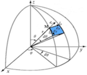
Figure 1. Tangent plane.

Note. We will find the geometrical and physical meaning of the functions coshη_α, sinhη_α, and tanhη_α in (12) and (14) (Figure 1) in the spherical coordinate system.

Also coshη_φ= (1-β²_φ)^-0.5

sinhη_φ=β_φ(1-β²_φ)^-0.5

tanhη_φ=β_φ

β_φ = v_φ /c. v_φ is the linear velocity of the system K

Since r is a straight line segment, the rotation in the plane t0r does not differ from the classical case:

coshη_r= (1-β²_r)^-0.5

sinhη_r=β_r(1-β²_r)^-0.5

β_r = v_r /c. v_r is the velocity along r.

3. Calculations

We will not give Lorentz transformations and wave aberrations in Cartesian coordinates. The reference of rotations on the t0x, t0y, t0z planes in Minkowski space where g₀₀ =1, g₁₁ = g₂₂ = g₃₃ = -1 and |τ_α0 |= I (– g₀₀ g_αα)^0.5= 1 can be found in

[13]

3.1. Lorentz Transformations and the Doppler Effect in the Time-Spherical Coordinate System: ct, r, θ, φ. (Figure 2)

Let us find the form of the Lorentz transformation (12) and the Doppler effect (14.1) in the time-spherical coordinate system: q⁰= ct is time or zero axis; q¹= r is the radius vector; q²= θ is zenith or polar angle; q³= φ is the azimuthal angle. 0 < t ≤ ∞, 0 ≤ r ≤ ∞, 0 ≤ θ ≤ π, 0 ≤ φ ≤ 2π.

Let α =3, i.e., x

Download: Download full-size image

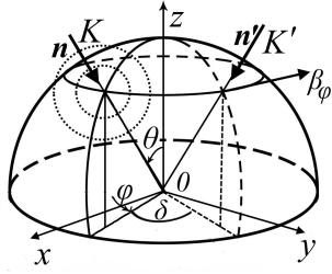
Figure 2. Wave aberration.

Then, from (12), we obtain the Lorentz transformations for the motion in the azimuthal plane with the velocity β_φ.

\{\begin{matrix} ct = (c t^{'} + r ∙ sinθ ∙ β_{φ} ∙ φ^{'}) / \sqrt{1 - β_{φ}^{2}} \\ φ = (φ^{'} + \frac{β_{φ}}{r ∙ sinθ} ∙ c t^{'}) / \sqrt{1 - β_{φ}^{2}} \end{matrix}

(15)

Let's find the type of Doppler effect and aberration. Our first objective is to determine the wave vector type for azimuthal motion β_φ (β_r = β_θ = 0) (Figure 3). βφ is a velocity of system K’ relative to K that is tangent to the arc (along φ).

Download: Download full-size image

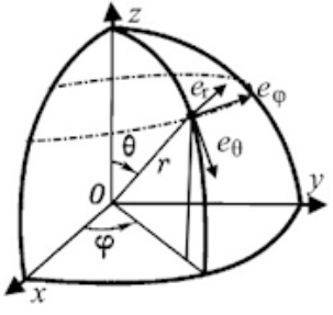
Figure 3. Body movement along axes.

The wave vector n is perpendicular to the front of a spherical monochromatic wave. The angle between n and x is equal to φ. The angle between vector n’ and x is equal to φ +δ.

The aberration angle δ is the angle between the vectors n and nʼ.

From equation (14) we get

\{\begin{matrix} ω^{'} = ω ∙ (1 - r ∙ sinθ ∙ β_{φ}) / \sqrt{1 - β_{φ}^{2}} \\ ω^{'} ∙ cosδ = ω ∙ (1 - \frac{β_{φ}}{r ∙ sinθ}) / \sqrt{1 - β_{φ}^{2}} \end{matrix}

(16)

The aberration angle δ is the difference between the angle of wave incidence from the source and the observed angle, which varies due to the rotation of the receiver (e.g., the Earth) in orbit.

(16.1) is the Lorentz transformation, and (16.2) is the aberration of the wave at the azimuthal velocity of the source (receiver). The aberration angle δ is defined relative to the wave vector n in formula (16.2).

We find δ relative to the observer (point 0) (Figure 3). Since ⦟z^n = φ and ⦟z^nʼ = φ + δ, then

k^{3} = \frac{ω}{c} cosφ

k^{' 3} = \frac{ω^{'}}{c} \cos (φ + δ)

k^{0} = \frac{ω}{c}

k^{' 0} = \frac{ω^{'}}{c}

Then equations (14) for α=3 can be written as:

ω^{'} = ω ∙ (\cosh η_{φ} - r ∙ sinθ ∙ cosφ ∙ \sinh η_{φ})

ω^{'} \cos (φ + δ) = ω (cosφ ∙ \cosh η_{φ} - \frac{1}{r ∙ sinθ} ∙ \sinh η_{φ})

Substituting the first equation into the second one, we get:

\cos (φ + δ) = \frac{cosφ - \frac{β_{φ}}{r ∙ sinθ}}{1 - r ∙ sinθ ∙ cosφ ∙ β_{φ}}

(17)

On the radial motion of the wave source or receiver (g₀₀ =1, g₁₁ = -1), we obtain the relativistic Einstein aberration formula

[14]

from (17).

If φ = π/2, then from (17) we get

sinδ = β_{φ} / r ∙ sinθ

(18)

Let's calculate the annual aberration of the stars. We take r =ρ/1au and θ = π/2 in formula (18).

1 au = 149 597 870 700 m is an astronomical unit.

On aphelion, the Earth's orbital velocity is βφ=29.29/3∙105, and it's ρ = 1.016 au from the Sun

[15]

. On perihelion, the Earth's orbital velocity is βφ=30.29/3∙105 and the distance to the Sun is ρ = 0.98329 au

[15]

Calculations using the formula (18) show that the annual aberration angle is equal to:

δ_a = 19.80753477^’’-for afelius; δ_p = 21.17978416^’’-for perihelion;

\overset{̅}{δ} = {20.49365946}^{''}

– mean value;

δ_exp =20.49552^’’ is the officially accepted annual aberration value

[16]

The measurement error (

Δ = (δ_{\exp} - \overset{̅}{δ}) / δ_{\exp}

) in the calculation of δ is less than Δ < 10^-3%.

We will not consider the case

α = 2

, i.e., motion along the direction of the vector e_θ(x^’0 = ct^’, x^’2 = θ^’, x⁰ = ct, x² = θ, g₀₀ =1, g₂₂ = -r², |τ₂₀| = r), since α = 2 is a special case of α = 3.

Also the case α = 1 (radial motion of the source and/or receiver) does not differ from the classical case (Cartesian coordinate system).

3.2. Hubble's Law

We now find the dependence of the redshift

z = (ω-ω^˺)/ω^˺ on the distance r between the source and receiver of the wave.

Substituting (16.1) into z, we get

z = \frac{sinθ ∙ β_{φ}}{1 - r ∙ sinθ ∙ β_{φ}} ∙ r

(19)

To be precise, the galaxy's recessional velocity v is by no means equal to, but only proportional to c∙z (the product of the speed of light c and the redshift z). Therefore, we multiply formula (19) by k∙c and obtain the dependence of the galaxy scattering velocity v on the distance between them r, i.e., Hubble's law

[17]

v = k ∙ c ∙ \frac{sinθ ∙ β_{φ} ∙ r}{1 - r ∙ sinθ ∙ β_{φ}}

(20)

For “small distances” (up to 4 Mpc), the coefficient k = 291.2583845 is determined by the least square method from the experiment

[20]

, which is given in Table 1 (light yellow columns).

Table 1. Experimental data for Hubble's law.

Experimental data for Hubble's law

from

[20]

from

[21]

from

[20]

[21]

-25

015.0

1380

000

-25

0.032

170

031.3

2304

000.032

170

0.034

290

038.7

3294

000.034

290

0.214

-130

039.5

3149

000.214

-130

0.263

-70

043.2

3272

000.263

-70

0.275

-202.5

045.1

3106

000.275

-202.5

0.45

200

050.9

4398

000.45

200

0.5

280

053.3

3545

000.5

280

0.62

300

056.0

4124

000.62

300

0.63

200

057.3

4869

000.63

200

0.67

400

058.0

4227

000.67

400

0.79

290

058.3

4061

000.79

290

0.8

300

062.2

4749

000.8

300

0.9

215.1665

066.6

4924

000.9

215.1665

760.

066.7

4730

001

760

1.1

537.5

066.8

4847

001.1

537.5

1.16

800

068.2

4820

001.16

800

1.2

580

071.8

5424

001.2

580

1.24

600

074.3

4982

001.24

600

1.27

730

077.9

5434

001.27

730

1.4

500

082.4

6673

001.4

500

1.42

700

085.6

7143

001.42

700

1.49

810

088.4

7016

001.49

810

1.52

650

088.6

5935

001.52

650

1.53

800

089.2

6709

001.53

800

1.7

960

096.7

7241

001.7

960

1.73

650

102.1

7765

001.73

650

1.74

940

114.9

8930

001.74

940

1.79

800

117.1

9801

001.79

800

810

119.7

8604

002

810

2.06

900

121.5

7880

002.06

900

2.23

1140

127.8

8691

002.23

1140

2.35

1100

132.7

10446

002.35

1100

2.37

1300

134.7

9065

002.37

1300

3.45

1800

136.0

9024

003.45

1800

149.9

10715

015.0

1380

151.4

10696

031.3

2304

158.9

12012

038.7

3294

176.8

12871

039.5

3149

183.9

13707

043.2

3272

185.6

14634

045.1

3106

19.80

1088

050.9

4398

198.6

15055

053.3

3545

20.70

1607

056.0

4124

202.3

14764

057.3

4869

202.5

13518

058.0

4227

215.4

15002

058.3

4061

235.9

17371

062.2

4749

236.1

15567

066.6

4924

238.9

16687

066.7

4730

262.2

18212

066.8

4847

274.6

22426

068.2

4820

280.1

18997

071.8

5424

303.4

21190

074.3

4982

309.5

23646

077.9

5434

391.5

26318

082.4

6673

467.0

30253

085.6

7143

088.4

7016

088.6

5935

089.2

6709

096.7

7241

102.1

7765

114.9

8930

117.1

9801

119.7

8604

121.5

7880

127.8

8691

132.7

10446

134.7

9065

136.0

9024

149.9

10715

151.4

10696

158.9

12012

176.8

12871

183.9

13707

185.6

14634

19.80

1088

198.6

15055

20.70

1607

202.3

14764

202.5

13518

215.4

15002

235.9

17371

236.1

15567

238.9

16687

262.2

18212

274.6

22426

280.1

18997

303.4

21190

309.5

23646

391.5

26318

467.0

30253

In (20), all variables (z, β_φ = v_φ/c, r) are dimensionless, so we accept r = d /R₀. R₀ = 14300 Mpc

[18]

is the radius of the effective particle horizon, up to which we can see particles created since the Big Bang;

d is the distance from the object to the observer, measured in Mpc;

β_{φ} = 24000 / 300000 = 0.08

is the linear velocity at the periapsis of S4714ʼs proper orbit

[19]

. This is the highest velocity in our galaxy (Milky Way).

Then (20) has the form (sinθ ≈ 1):

/ ( v=0.08k∙cdR₀-0.08d)(21)

Figure 4 shows the approximation of the data from

[20]

by function (21). ∎-data from

[20]

, red dashed line-function (21). We can see that formula (21) agrees well with experiments up to distances d ∼4 Mpc.

Download: Download full-size image

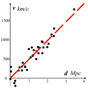
Figure 4. Hubble’s law.

If we consider Hubble's law as before, i.e., the dependence v∼ f(d) is linear (Figure 5)

v = H (r, θ, v_φ) ∙ d,

then we get the Hubble parameter H (r, θ, v_φ):

H (d, θ, v_{φ}) = \frac{sinθ ∙ β_{φ} ∙ k ∙ c}{1 - sinθ ∙ β_{φ} ∙ d}

(22)

Download: Download full-size image

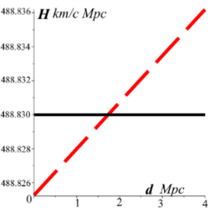
Figure 5. Hubble parameter.

here

\overset{̅}{H} = 488.83

In fact, H (r, θ, v_φ) depends on d, θ, and v_φ. Therefore, the Hubble parameter grows weakly with increasing source-receiver distance (Figure 5).

It would be more correct to take the dependence z∼ f (d) instead of v ∼ f (d). Hubble's law was originally derived empirically, also from the assumption that the redshift of the spectrum is due to the radial velocity of objects. In addition, the assumption was that the dependence would be linear. But formula (21) shows that Hubble's law is nonlinear: as the distance between objects increases, the “galaxy expanding velocity,” or more precisely, the redshift (Hubble parameter, too), increases even at low velocities and without radial velocity, i.e., without galaxy expansion (v_r= 0).

At large distances (up to 500 Mpc), the redshift and the Hubble parameter increase further (Figure 6), red dotted line).

The small inside figure is a Hubble diagram. The red square at the origin shows the comparative scale and location of the Hubble diagram.

Download: Download full-size image

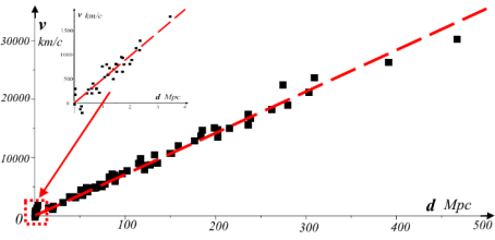
Figure 6. Hubble's Law at Long Distances.

The function (21) tends to infinity, i.e., it will have a singularity at 0.08 d → R₀.

For distances (up to 500 Mpc), the coefficient k =42.21890063 is determined by the least square method from the experiment

[20, 21]

, which is given in Table 1 (light blue columns).

The cause of redshift is not only radial motion but also an orbital motion of the source and/or receiver. Simply put, the radial recede of galaxies is not the main reason for redshift. The source and/or receiver's orbital motion is likely the primary cause of the redshift.

Now consider the dependence of redshift z on the zenith angle θ and the distance between objects d: z∼ f (d, θ).

From (20) we get

z = \frac{k ∙ sinθ ∙ 0.08}{R_{0} - sinθ ∙ 0.08 ∙ d} ∙ d

(23)

Figure 7 shows the dependence: z∼ f (d, θ). The two-dimensional plot (Figure 7A) shows that z reaches a maximum at θ = π/2 for all values of d (d₁>d₂>d₃>d₄). Astronomers often take the angle θ (zero) not from the North Pole

[22]

, but from the ecliptic plane, i.e., from the plane of the Earth's orbit around the Sun. Then we should use cosθ instead of sinθ in formula (23). We'll continue that tradition.

Download: Download full-size image

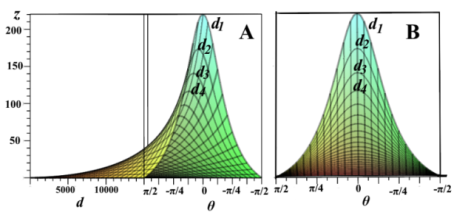
Figure 7. Dependence z∼ f(d, θ) and its section by d.

Figure 7B shows the projection of f (d, θ) onto the z, θ plane. The graph shows that the closer the angle θ is to the ecliptic (θ→ 0) and the larger the distance d, the larger the redshift z.

We can only observe longitude 0 ≤ φ ≤ 2π and latitude –π/2 ≤ θ ≤ 2π in the sky. We don't see the depth of the sky, i.e., the distance d to the celestial object. We determine it by indirect evidence (brightness, etc.). We calculate the redshift z by formula (23). However, formula (23) depends not on angle φ but on angle θ (Figure 7B).

If the dependence z∼ f (d, θ) (24) is plotted on a map of the Universe (latitude and longitude), we get the picture as in Figure 8A.

Figure 8B shows a map of the anisotropy of the relic radiation

[23]

in the K, Ka, Q, V, and W bands. A plot of z versus zenith angle θ (- 900 ≤ θ ≤900 vertically) on the latitude-longitude map is shown on the left (Figure 8A).

We see that the z maxima are centered on a narrow band for all d (red shaded band in Figure 8A). In the experiment, the "hot" (red) regions are also located in the center of the ecliptic (Figure 8B).

Download: Download full-size image

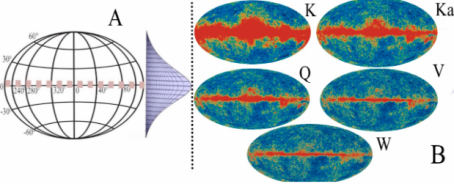
Figure 8. Universe map in latitudes and longitudes.

We see that the z maxima are centered on a narrow band for all d (red shaded band in Figure 8A). In the experiment, the "hot" (red) regions are also located in the center of the ecliptic (Figure 8B) (Figure 8В). Simply put, the observer (telescope) fixes large ("hot") z 's closer to the ecliptic and small ("cold") z 's farther from the ecliptic. This is similar to how an astronaut from space cannot tell the height of mountain ranges on Earth but only sees stripes where the ridges are.

Note again that the width and length of the red shaded band (Figure 8A) depend on z: narrow and short bands correspond to large z, and wide and long bands correspond to small z. This is visually consistent with the data on the right: K <Ka <Q <V <W.

The irregularity of the bands in Figure 8B (randomness, scattering) is most likely due to the random distribution of the object velocity and the proximity of the clusters. The "disorderly" arrangement of bright points in cold regions (further from the ecliptic) is probably due to a random distribution of distances d between the source and the receiver (observer).

3.3. Polarization of the Waves

The wave vector changes direction relative to the observer due to the satellite's orbital rotation. The direction of the wave vector changes by an angle δ (aberration angle) due to the rotation of the stars in their orbits and/or the rotation of the Earth around the Sun. The rotation of the source and/or receiver along the orbit is the cause of the change in the direction of the wave vector, causing the change from n to n^’. This change in the direction of the wave is the cause of the transverse Doppler effect, the aberration, and the polarization of the "refracted" wave.

By analogy with geometrical optics in formula (17), we denote:

π/2-φ = α is the angle of incidence of the wave; π/2-(φ+δ) = γ is the angle of refraction of the wave;

Considering

cos (φ + δ) = cos (π/2 - γ) = sinγ and

cosφ = cos (π/2 - α) = sinα

and simplifying from equation (17), we get

\frac{sinα}{sinγ} = \frac{1 - r ∙ sinθ ∙ sinα ∙ β_{φ}}{1 - β_{φ /} r ∙ sinθ ∙ sinα}

Let θ = π/2. Then

\frac{sinα}{sinγ} = \frac{1 - r ∙ sinα ∙ β_{φ}}{1 - \frac{β_{φ}}{r ∙ sinα}}

(24)

By analogy with Snell's law

[24]

, let us introduce the "refractive index" of the vacuum:

n = \frac{1 - r ∙ sinα ∙ β_{φ}}{1 - \frac{β_{φ}}{r ∙ sinα}}

(25)

If g₃₃ = r∙ sinα = -1 (rectangular coordinates), then (25) gives n=1– the classical "refractive index" of vacuum. In curvilinear coordinates, the refractive index of vacuum

n

differs from unity. For example, for an observer on Earth at aphelion n=0.9999967655 < 1, at perihelion n = 1.000003403 > 1.

Let the "incident" monochromatic wave n be directed along the unit vector k and the velocity of the wave source be along the unit vector j. The direction of the "refracted" wave n^’ will be k^’, and the direction of the velocity n^’ will be j^’ (Figure 9).

Download: Download full-size image

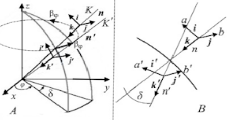
Figure 9. Wave polarization.

Figure 9A shows the incident wave K and the wave K^’(with velocity β_φ on orbit) in a spherical coordinate system. Figure 9B shows the waves Κ and Κ^’ on the incision plane through a vertical plane (the azimuthal angle is φ). Note that j and j^’ coincide.

We directed n along k freely, at our discretion, and the velocity

β_{φ}

along j. But the choice of kʼ, jʼ, and iʼ is not free, but rigidly connected with k, j, and i.

Let's consider the electrical components of the "incident" wave:

E = E_{0} e^{i (k r - ωt)} = E_{0} \cos (k r - ωt) + i E_{0} \sin (k r - ωt)

k

is the wave vector.

Of course, all of the above also applies to the magnetic field.

Let’s introduce vectors:

a = E_{0} \cos (k r - ωt) = ia

;

b = Re {i E_{0} \sin (k r - ωt)} = jb

;

a^{'} = E_{0}^{'} \cos (k r - ωt) = i a^{'}

;

b^{'} = Re {i E_{0}^{'} \sin (k r - ωt)} = j b^{'}

Then E = i ∙a +j ∙b, E^’ = i^'∙a^’ +j^’∙b^’

Figure 9B clearly shows that the angle between a and aʼ is equal to

δ

, as is the angle between i^iʼ and between k^kʼ. The angle between b and bʼ is zero, as is the angle between j^jʼ.

The projections of aʼ onto a and bʼ onto b are:

a^'ʹ= a∙ cosδ and b^’ʹ=b

The polarization vector is along k. Since we have described n in the right-handed coordinate system (right-handed vector triad), nʼ will also be right-handed polarized.

Let's find the polarization vector P (a=b):

P = \frac{E_{j}^{2} - E_{i}^{2}}{E_{j}^{2} + E_{i}^{2}} = \frac{b^{2} - a^{2} \cos^{2} δ}{b^{2} + a^{2} \cos^{2} δ}

Incident wave (n) is natural, not polarized. For natural light, where waves of different polarizations are equally mixed and all directions are equal. Assuming that the polarized wave nˈ (after "refraction") is half the natural wave, we get:

P = \frac{1}{2} ∙ \frac{1 - \cos^{2} δ}{1 + \cos^{2} δ}

(26)

From formula (26), we can find the degree of polarization for annual aberration. Substituting (18) into (26) and simplifying, we get:

P = \frac{1}{2} ∙ \frac{\sin^{2} δ}{2 - \sin^{2} δ} = \frac{0.5}{2 ∙ \sin^{- 2} δ - 1}

P = \frac{0.5}{2 ∙ β_{φ}^{- 2} ∙ r^{2} ∙ \cos^{2} θ - 1}

(27)

At aphelion (β_φ=29.29/300000, r=1.0167 au, θ = 0)-P_α = 2.31∙10^-9. At perihelion (β_φ=30.29/300000, r=0.98329 au, θ = 0)-P_p = 2.64∙10^-9.

We took the zenith angle from the ecliptic, following the astronomers: sinθ → cosθ. Of course, the effects are very weak: P_α and P_p.

In general, the degree of polarization (27) depends on the distance between the source and receiver and the zenith angle (elevation angle).

The starlight polarization dependence denoted as

P = ∣ \frac{k ∙ 0.5}{2 ∙ β_{φ}^{- 2} ∙ {(d / R_{0})}^{2} ∙ \cos^{2} θ - 1} ∣

,(28)

is illustrated in Figure 10.

Download: Download full-size image

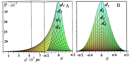
Figure 10. Starlight polarization dependence P = f (d, θ).

βφ = 10^-4 is Earth's average orbital velocity; R₀ =14300∙106 pc

[18]

; d is distance from observer (on Earth) to wave source.

k=0.03.

The degree of polarization, P, of the starlight at the moment of emission (at the beginning) is unknown. According to observations reported in

[25]

, the degree of polarization is approximately 1.5% for stars at a distance of 1000 parsecs. Therefore, the coefficient of proportionality is taken to be k = 0.03.

It is important to note that the graphs depicted in Figure 10 of the study on starlight polarization should not be regarded as a quantitative analysis in the strict sense of the term. Rather, they serve as a visual representation of the trends in the laws of starlight polarization.

The dependences of P∼ f(θ) at d₁ > d₂ > d₃ > d₄ are shown in Figure 10B.

Figure 10B is an incision of the 3-dimensional Figure 10A by the plane θ: P∼ f (d, θ). It is obvious that for large d and θ ∼ 0, the degree of polarization P is maximum.

Figure 11 shows plots of experimental data on measurements of the degree of polarization of stars

[25]

Download: Download full-size image

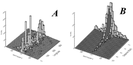
Figure 11. Experimental data of the polarized starlight.

Graph 10A does not conflict with Graph 11B, which is the experiment. Graph 11A doesn’t contradict Graph 10B if the latter is placed on the θ, φ plane.

It is obvious that here, as in the case of the redshift (Figure 8), we also see a stripe close to the ecliptic (θ∼0) (Figure 10).

Download: Download full-size image

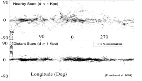
Figure 12. CMB polarization.

Figure 12 shows starlight polarization vectors in galactic coordinates for 5513 stars. {52} for a local cloud (upper) and for an average polarization vector over many clouds (lower).

Our calculations for measuring the degree of polarization do not include statistical hypothesis testing (due to the small sample). Nevertheless, both graphs (Figures 11 and 12) visually demonstrate the correctness of our assumption about the dependence of the degree of polarization on distance and polar angle: the greater the distance between the source and receiver of the wave and the closer the elevation angle to the ecliptic (

θ ~ 0

), the greater the degree of polarization. In other words, large redshifts z and maximum degrees of polarization P are concentrated near the ecliptic plane.

Abbreviations

CMB	Cosmic Microwave Background
pc	Parsec
Mpc	Mega Parsec

Acknowledgments

It should be noted that I would hardly be able to compare with reality and check the plausibility of the theoretical assumptions presented in the article without the scientific works (without experimental data) of scientists such as Hubble E., Freedman W. L. and co-authors, Rosalia P., Lazarian Alex and co-authors, and also Bennett et al.

I would like to express my gratitude to my ally, my wife Lyuba Gomazkova, for correcting and formatting the Russian version of the text and formulas, for creating a cozy and comfortable working environment, and, above all, for her angelic patience.

I would like to express special thanks to SciencePG for their unpaid help and work in publishing this (not only this) article. They have become the "godfathers" of my articles for the English-speaking public.

Author Contributions

Alimzhan Kholmuratovich Babaev is the sole author. The author read and approved the final manuscript.

Conflicts of Interest

The author declares no conflicts of interest.

References

[1]	Daniel Nieto Yll. Doppler shift compensation strategies for LEO satellite communication systems. Polytechnic University of Catalonia. Published 1 June 2018. https://upcommons.upc.edu/bitstream/handle/2117/123510/DanielNietoYll_Doppler_compensation_for_LEO.pdf
[2]	The global positioning system, relativity, and extraterrestrial navigation Neil Ashby and Robert A. Nelson 2008. https://doi.org/10.1017/S174392130999010X
[3]	Wikipedia. Lorentz transformations. https://en.wikipedia.org/wiki/Lorentz_transformation
[4]	Pain, Reynald; Astier, Pierre (2012). "Observational evidence of the accelerated expansion of the Universe". Comptes Rendus Physique. 13 (7): 521–538. pp. 13-16 https://doi.org/10.1016/j.crhy.2012.04.009 (In French).
[5]	Jacques Colin, Roya Mohayaee, Mohamed Rameez and Subir Sarkar (Nov 2019). "Evidence for anisotropy of cosmic acceleration⋆". Astronomy & Astrophysics. 631: L13. https://doi.org/10.1051/0004-6361/201936373 20.11. 2019.
[6]	Freedman, W. L.; Madore, B. F. (2010). The Hubble Constant. Annual Review of Astronomy and Astrophysics. 48: 673–710. https://doi.org/10.48550/arXiv.1004.1856
[7]	Sangwine, Stephen J.; Ell, Todd A.; Le Bihan, Nicolas (2010), "Fundamental representations and algebraic properties of biquaternions or complexified quaternions", Advances in Applied Clifford Algebras, 21 (3): 1–30, https://doi.org/10.48550/arXiv.1001.0240
[8]	The rules of 4-dimensional perspective: How to implement Lorentz transformations in relativistic visualization. Andrew J. S. Hamilton. [gr-qc] 16 Nov 2021. https://doi.org/10.1007/s00006-022-01257-5
[9]	Babaev A. Kh., Biquaternions, rotations, and spinors in the generalized Clifford algebra (in Russian). Sci-article.ru. № 45 (May) 2017. pp. 296 - 304, https://doi.org/10.24108/preprints-3112462
[10]	Chris J. L. Doran. Geometric Algebra and its Application to Mathematical Physics. Sidney Sussex College. A dissertation submitted for the degree of Doctor of Philosophy in the University of Cambridge. February 1994, pages 4-6.
[11]	Gaston Casanova. L’Algebre Vectorielle. Press Universitaires de France. p. 10, 19. https://books.google.ru/books?id=Es__EAAAQBAJ&pg=PA2&hl=ru&source=gbs_toc_r&cad=2#v=onepage&q&f=false
[12]	Babaev A. Kh. Alternative formalism based on Clifford algebra (in Russian), SCI-ARTICLE.RU. №40 (December) 2016, pp. 34-42, https://doi.org/10.24108/preprints-3112477
[13]	Landau L. D., Lifshitz E. M., The Classical Theory of Fields, Course of Theoretical Physics, vol. 2, pp. 123-127.
[14]	Albert Einstein (1905) "Zur Elektrodynamik bewegter Körper", Annalen der Physik 17: 891; English translation. https://doi.org/10.1002/andp.19053221004
[15]	Wikipedia. https://en.wikipedia.org/wiki/Earth%27s_orbit
[16]	Wikipedia. https://en.wikipedia.org/wiki/Astronomical_constant
[17]	Dan Scolnic, Lucas M. Macri, Wenlong Yuan, Stefano Casertano, Adam G. Riess. Large Magellanic Cloud Cepheid Standards Provide a 1% Foundation for the Determination of the Hubble Constant and Stronger Evidence for Physics Beyond Lambda CDM -2019-03-18. https://doi.org/10.48550/arXiv.1903.07603
[18]	Gott III, J. Richard; Mario Jurić; David Schlegel; Fiona Hoyle; et al. (2005). "A Map of the Universe" (PDF). The Astrophysical Journal. 624 (2): 463–484. https://doi.org/10.1086/428890
[19]	Florian Peißker, Andreas Eckart, Michal Zajaček, Basel Ali, Marzieh Parsa. S62 and S4711: Indications of a population of faint fast moving stars inside the S2 orbit -- S4711 on a 7.6 year orbit around Sgr~A* // The Astrophysical Journal. — 2020-08-11. https://doi.org/10.48550/arXiv.2008.04764
[20]	Hubble E. (1929). "A relation between distance and radial velocity among extra-galactic nebulae". Proceedings of the National Academy of Sciences 15 (3): 168–173. https://doi.org/10.1073/pnas.15.3.168
[21]	W. L. Freedman, B. F. Madore, B. K. Gibson, L. Ferrarese, D. D. Kelson, S. Sakai, J. R. Mould, R. C. Kennicutt Jr., H. C. Ford, J. A. Graham and others, Hubble, E. (1929). "A relation between distance and radial velocity among extra-galactic nebulae". Proceedings of the National Academy of Sciences. 15 (3): 168–173. Final Results from the Hubble Space Telescope Key Project to Measure the Hubble Constant, https://doi.org/10.48550/arXiv.astro-ph/0012376
[22]	Wikipedia. https://en.wikipedia.org/wiki/Ecliptic
[23]	First Year Wilkinson Microwave Anisotropy Probe (WMAP) Observations: Preliminary Maps and Basic Results, C.L. Bennett, et al., 2003ApJS..148....1B, reprint / preprint (4.4 Mb) / individual figures / ADS / astro-ph, https://lambda.gsfc.nasa.gov/product/wmap/pub_papers/firstyear/basic/wmap_cb1_images.html
[24]	Wikipedia. https://en.wikipedia.org/wiki/Snell%27s_law
[25]	Fosalba, Pablo; Lazarian, Alex; Prunet, Simon; Tauber, Jan A. (2002). "Statistical Properties of Galactic Starlight Polarization". Astrophysical Journal. 564 (2): 762–772. https://doi.org/10.1086/324297

Cite This Article

Plain Text BibTeX RIS

APA Style

Babaev, A. K. (2025). Description of Lorentz Transformations, the Doppler Effect, Hubble's Law, and Related Phenomena in Curvilinear Coordinates by Generalized Biquaternions. American Journal of Astronomy and Astrophysics, 12(1), 9-20. https://doi.org/10.11648/j.ajaa.20251201.12

Copy | Download

ACS Style

Babaev, A. K. Description of Lorentz Transformations, the Doppler Effect, Hubble's Law, and Related Phenomena in Curvilinear Coordinates by Generalized Biquaternions. Am. J. Astron. Astrophys. 2025, 12(1), 9-20. doi: 10.11648/j.ajaa.20251201.12

Copy | Download

AMA Style

Babaev AK. Description of Lorentz Transformations, the Doppler Effect, Hubble's Law, and Related Phenomena in Curvilinear Coordinates by Generalized Biquaternions. Am J Astron Astrophys. 2025;12(1):9-20. doi: 10.11648/j.ajaa.20251201.12

Copy | Download

@article{10.11648/j.ajaa.20251201.12,
  author = {Alimzhan Kholmuratovich Babaev},
  title = {Description of Lorentz Transformations, the Doppler Effect, Hubble's Law, and Related Phenomena in Curvilinear Coordinates by Generalized Biquaternions},
  journal = {American Journal of Astronomy and Astrophysics},
  volume = {12},
  number = {1},
  pages = {9-20},
  doi = {10.11648/j.ajaa.20251201.12},
  url = {https://doi.org/10.11648/j.ajaa.20251201.12},
  eprint = {https://article.sciencepublishinggroup.com/pdf/10.11648.j.ajaa.20251201.12},
  abstract = {This paper presents the derivation of Lorentz transformations in curvilinear coordinates utilizing generalized biquaternions. Generalized biquaternions are rotations in curvilinear coordinates, including on the tx, ty, and tz planes. These space-time rotations are precisely the Lorentz transformations in curvilinear coordinates. The orbital rotation of the source and/or receiver, which mathematically represents the Lorentz transformation in spherical coordinates, is identified as the cause of the transverse Doppler effect. The change in wave frequency, specifically the "redshift," results in nonlinearities of Hubble's law manifesting as phenomena such as accelerated and anisotropic expansion of the universe, aberration, and wave polarization. Apparently, redshift exists even without radial expansion of the universe, i.e., without the "Big Bang". The reasons for the accelerated expansion of the universe, the anisotropic (angular) distribution of relic radiation, and the polarization of light from distant stars become clear in this approach. This greatly simplifies the mathematical description and understanding of the supposedly complex processes occurring in the universe.},
 year = {2025}
}

Copy | Download

TY  - JOUR
T1  - Description of Lorentz Transformations, the Doppler Effect, Hubble's Law, and Related Phenomena in Curvilinear Coordinates by Generalized Biquaternions
AU  - Alimzhan Kholmuratovich Babaev
Y1  - 2025/01/22
PY  - 2025
N1  - https://doi.org/10.11648/j.ajaa.20251201.12
DO  - 10.11648/j.ajaa.20251201.12
T2  - American Journal of Astronomy and Astrophysics
JF  - American Journal of Astronomy and Astrophysics
JO  - American Journal of Astronomy and Astrophysics
SP  - 9
EP  - 20
PB  - Science Publishing Group
SN  - 2376-4686
UR  - https://doi.org/10.11648/j.ajaa.20251201.12
AB  - This paper presents the derivation of Lorentz transformations in curvilinear coordinates utilizing generalized biquaternions. Generalized biquaternions are rotations in curvilinear coordinates, including on the tx, ty, and tz planes. These space-time rotations are precisely the Lorentz transformations in curvilinear coordinates. The orbital rotation of the source and/or receiver, which mathematically represents the Lorentz transformation in spherical coordinates, is identified as the cause of the transverse Doppler effect. The change in wave frequency, specifically the "redshift," results in nonlinearities of Hubble's law manifesting as phenomena such as accelerated and anisotropic expansion of the universe, aberration, and wave polarization. Apparently, redshift exists even without radial expansion of the universe, i.e., without the "Big Bang". The reasons for the accelerated expansion of the universe, the anisotropic (angular) distribution of relic radiation, and the polarization of light from distant stars become clear in this approach. This greatly simplifies the mathematical description and understanding of the supposedly complex processes occurring in the universe.
VL  - 12
IS  - 1
ER  -

Copy | Download

Author Information

Alimzhan Kholmuratovich Babaev

Department Physics, National University of Uzbekistan, Tashkent, Republic of Uzbekistan; Department of Applied Mathematics and Computer Science, Novosibirsk State Technical University, Novosibirsk, Russian Federation

Biography: Alimzhan Kholmuratovich Babaev defended his thesis for a PhD in physical and math sciences on the topic “Multiple collisions of particles and fragmentations of 22Ne nuclei in a photoemulsion at P/A=4.1 GeV/c” in 1989 at the Institute of Nuclear Physics of the Academy of Sciences of Uzbekistan (Tashkent). He worked at the Department of Nuclear Physics and Cosmic Rays at the National University (Tashkent, Uzbekistan) as an associate professor. Since 2000, he has worked as a lecturer at the Novosibirsk State Technical University (Novosibirsk, Russian Federation) in the Department of Higher Mathematics. At present, he is working as an independent researcher in the field of applications of methods of abstract algebra to classical and quantum field physics. He is the author (co-author) of more than 30 scientific papers published in peer-reviewed journals.

Research Fields: Research field: Clifford algebra, Gravity, Electromagnetism, Biquaternions and Spinor fields, Partial differential equations, Unified field theory.

Contact Email

http://orcid.org/0000-0002-4071-5524

Download PDF

Table 1

Table 1. Experimental data for Hubble's law.

Plain Text BibTeX RIS

APA Style

Babaev, A. K. (2025). Description of Lorentz Transformations, the Doppler Effect, Hubble's Law, and Related Phenomena in Curvilinear Coordinates by Generalized Biquaternions. American Journal of Astronomy and Astrophysics, 12(1), 9-20. https://doi.org/10.11648/j.ajaa.20251201.12

Copy | Download

ACS Style

Babaev, A. K. Description of Lorentz Transformations, the Doppler Effect, Hubble's Law, and Related Phenomena in Curvilinear Coordinates by Generalized Biquaternions. Am. J. Astron. Astrophys. 2025, 12(1), 9-20. doi: 10.11648/j.ajaa.20251201.12

Copy | Download

AMA Style

Babaev AK. Description of Lorentz Transformations, the Doppler Effect, Hubble's Law, and Related Phenomena in Curvilinear Coordinates by Generalized Biquaternions. Am J Astron Astrophys. 2025;12(1):9-20. doi: 10.11648/j.ajaa.20251201.12

Copy | Download

@article{10.11648/j.ajaa.20251201.12,
  author = {Alimzhan Kholmuratovich Babaev},
  title = {Description of Lorentz Transformations, the Doppler Effect, Hubble's Law, and Related Phenomena in Curvilinear Coordinates by Generalized Biquaternions},
  journal = {American Journal of Astronomy and Astrophysics},
  volume = {12},
  number = {1},
  pages = {9-20},
  doi = {10.11648/j.ajaa.20251201.12},
  url = {https://doi.org/10.11648/j.ajaa.20251201.12},
  eprint = {https://article.sciencepublishinggroup.com/pdf/10.11648.j.ajaa.20251201.12},
  abstract = {This paper presents the derivation of Lorentz transformations in curvilinear coordinates utilizing generalized biquaternions. Generalized biquaternions are rotations in curvilinear coordinates, including on the tx, ty, and tz planes. These space-time rotations are precisely the Lorentz transformations in curvilinear coordinates. The orbital rotation of the source and/or receiver, which mathematically represents the Lorentz transformation in spherical coordinates, is identified as the cause of the transverse Doppler effect. The change in wave frequency, specifically the "redshift," results in nonlinearities of Hubble's law manifesting as phenomena such as accelerated and anisotropic expansion of the universe, aberration, and wave polarization. Apparently, redshift exists even without radial expansion of the universe, i.e., without the "Big Bang". The reasons for the accelerated expansion of the universe, the anisotropic (angular) distribution of relic radiation, and the polarization of light from distant stars become clear in this approach. This greatly simplifies the mathematical description and understanding of the supposedly complex processes occurring in the universe.},
 year = {2025}
}

Copy | Download

TY  - JOUR
T1  - Description of Lorentz Transformations, the Doppler Effect, Hubble's Law, and Related Phenomena in Curvilinear Coordinates by Generalized Biquaternions
AU  - Alimzhan Kholmuratovich Babaev
Y1  - 2025/01/22
PY  - 2025
N1  - https://doi.org/10.11648/j.ajaa.20251201.12
DO  - 10.11648/j.ajaa.20251201.12
T2  - American Journal of Astronomy and Astrophysics
JF  - American Journal of Astronomy and Astrophysics
JO  - American Journal of Astronomy and Astrophysics
SP  - 9
EP  - 20
PB  - Science Publishing Group
SN  - 2376-4686
UR  - https://doi.org/10.11648/j.ajaa.20251201.12
AB  - This paper presents the derivation of Lorentz transformations in curvilinear coordinates utilizing generalized biquaternions. Generalized biquaternions are rotations in curvilinear coordinates, including on the tx, ty, and tz planes. These space-time rotations are precisely the Lorentz transformations in curvilinear coordinates. The orbital rotation of the source and/or receiver, which mathematically represents the Lorentz transformation in spherical coordinates, is identified as the cause of the transverse Doppler effect. The change in wave frequency, specifically the "redshift," results in nonlinearities of Hubble's law manifesting as phenomena such as accelerated and anisotropic expansion of the universe, aberration, and wave polarization. Apparently, redshift exists even without radial expansion of the universe, i.e., without the "Big Bang". The reasons for the accelerated expansion of the universe, the anisotropic (angular) distribution of relic radiation, and the polarization of light from distant stars become clear in this approach. This greatly simplifies the mathematical description and understanding of the supposedly complex processes occurring in the universe.
VL  - 12
IS  - 1
ER  -

Copy | Download