This paper explores the feasibility and effectiveness of using the Fengyun-3 meteorological satellite to monitor sea ice, providing services for ships navigating in polar regions. Firstly, it analyzes the impact of Arctic sea ice changes on ship navigation and the importance of sea ice monitoring in route planning. Next, it provides a detailed introduction to the data sources and processing methods of the Fengyun-3 satellite, including radiometric calibration, geometric correction, image registration, and cropping. Subsequently, it discusses the characteristics of sea ice in the visible spectrum and successfully extracts sea ice information using MERSI-II data with land, cloud, and seawater masking techniques. The study indicates that the comprehensive use of multi-spectral data and other observation methods can significantly enhance sea ice monitoring capabilities. In the future, integrating more advanced technologies is expected to achieve refined identification and short-term prediction of sea ice movement, thereby providing more scientific and efficient support for ships navigating in polar regions, enhancing navigation safety and efficiency, and offering a scientific basis for the development of Arctic shipping routes.
| Published in | American Journal of Traffic and Transportation Engineering (Volume 9, Issue 5) |
| DOI | 10.11648/j.ajtte.20240905.13 |
| Page(s) | 89-97 |
| Creative Commons |
This is an Open Access article, distributed under the terms of the Creative Commons Attribution 4.0 International License (http://creativecommons.org/licenses/by/4.0/), which permits unrestricted use, distribution and reproduction in any medium or format, provided the original work is properly cited. |
| Copyright |
Copyright © The Author(s), 2024. Published by Science Publishing Group |
Sea Ice Monitoring, Fengyun-3 Satellite, Polar Navigation, Remote Sensing Technology
Data Level | Abbreviation | Classification Principle |
|---|---|---|
Level 0 | L0 | Raw satellite data received by the ground system |
Level 1 | L1 | Basic data obtained from Level 0 data after quality inspection, image positioning, and radiometric calibration |
Level 2 | L2 | Various application data obtained from Level 1 data through projection transformation, inversion, or other calculations |
Level 3 | L3 | Statistical data obtained from Level 2 data through time averaging, accumulation, or analysis data obtained through human-computer interaction |
Level 4 | L4 | Reanalysis data generated using Level 2 or Level 3 data and various weather and climate model products |
 (1)
(1)  (5)
(5) FY-3 | Fengyun-3 |
MERSI | Medium Resolution Spectral Imager |
NDSI | Normalized Difference Snow Index |
NDVI | Normalized Difference Vegetation Index |
SAR | Synthetic Aperture Radar |
SSM/I | Special Sensor Microwave/Imager |
AMSR-2 | Advanced Microwave Scanning Radiometer-2 |
NSIDC | National Snow and Ice Data Center |
IFREMER | French Research Institute for the Exploitation of the Seas |
OSI-SAF | Ocean and Sea Ice Satellite Application Facility |
GIS | Geographic Information System |
L0 | Level 0 |
L1 | Level 1 |
L2 | Level 2 |
L3 | Level 3 |
L4 | Level 4 |
EV | Earth View |
| [1] | Andrews, J., Babb, D., & Barber, D. G. (2018). Climate change and sea ice: Shipping in Hudson Bay, Hudson Strait, and Foxe Basin (1980–2016). Elementa: Science of the Anthropocene, 6, 19. |
| [2] | Kiiski, T. (2017). Feasibility of Commercial Cargo Shipping along the Northern Sea Route. |
| [3] | Zhang, W., Wang, Y., Mou, C. R., et al. (2024). Route planning for the Arctic Northeast Passage considering multiple risk factors. Journal of Dalian Maritime University, 50(02), 1-10. |
| [4] | Lan, Q., & Zhang, X. (2024). Development of the Arctic route under the Belt and Road Initiative: Drivers, trends, and China's response. Journal of Beijing Jiaotong University (Social Sciences Edition), 1-15. [2024-09-26]. |
| [5] | Wang, H., Li, Z., Li, C., et al. (2024). Opportunities, challenges, and responses for China regarding the construction of the Arctic route. International Economic Cooperation, 40(04), 67-76+94. |
| [6] | Fang, Y., Wang, X., Chen, Z. Q., et al. (2023). Analysis of summer sea ice drift and changes in the Fram Strait from 2011 to 2020. Acta Geophysica, 66(07), 2726-2740. |
| [7] | Liang, S. (2021). Research on remote sensing inversion methods for polar sea ice density and thickness. University of Chinese Academy of Sciences (Institute of Space Information Innovation, Chinese Academy of Sciences). |
| [8] | Yan, Q., & Huang, W. (2019). Sea Ice Remote Sensing Using GNSS-R: A Review. Remote Sens. 11, 2565. |
| [9] |
Zhang, X., Fang, H. L., Wang, R. F., et al. (2024). Inversion method for Arctic thin ice thickness based on FY-3D microwave imager. Advances in Marine Science, 1-13. [2024-09-26].
http://kns.cnki.net/kcms/detail/37.1387.P.20240604.0956.002.html |
| [10] | Zheng, M. W., Li, X. M., & Ren, Y. Z. (2018). Research on automatic detection methods for polar sea ice using Synthetic Aperture Radar from GaoFen-3. Acta Oceanologica Sinica, 40(09), 113-124. |
| [11] | Zhao, C. F., Xu, R., & Zhao, K. (2019). Research on polar sea ice detection methods based on HY-2A/SCAT data. Journal of Ocean University of China (Natural Science Edition), 49(10), 140-149. |
| [12] | Kharbouche, S., & Muller, JP. (2019). Sea Ice Albedo from MISR and MODIS: Production, Validation, and Trend Analysis. Remote Sensing, 11(1), 9. |
| [13] | Zhou, Y., Kuang, D. B., & Gong, C. L., et al. (2017). Method for extracting Arctic sea ice parameters from MERSI images of Fengyun-3 satellite. Journal of Infrared and Millimeter Waves, 36(01), 41-48+126-127. |
| [14] | Yang, Z. J., Wang, Z. M., & Liu, T. T. (2023). Accuracy assessment of estimating Arctic sea ice area and edge using microwave data from Fengyun-3D. Polar Research, 35(01), 46-58. |
| [15] | Miao, S. X., Sun, K. M., Hu, X. Q., et al. (2024). Analysis of monitoring capabilities for plateau lake range based on MERSI-II images from Fengyun-3D. Journal of Wuhan University (Information Science Edition), 1-15. [2024-08-18]. |
| [16] |
China Meteorological Administration. (2018). [Online]. Available:
https://www.cma.gov.cn/zfxxgk/gknr/wjgk/gfxwj/201808/t20180820_1711977.html |
| [17] | Zhang, J. W., & Qiu, Z. F. (2021). Quality assessment of FY-3D MERSI II data for oceanic water areas. Acta Optica Sinica, 41(12), 19-38. |
| [18] | Zhu, X. Y., Su, J., Song, M., et al. (2022). Optimization of the algorithm for retrieving ice thickness in the Bohai Sea based on MODIS data. Acta Oceanologica Sinica, 44(12), 70-83. |
| [19] | Riggs, G. A., Hall, D. K., & Ackerman, S. A. (1999). Sea ice extent and classification mapping with the Moderate Resolution Imaging Spectroradiometer Airborne Simulator. Remote Sensing of Environment, 68(2), 152-163. |
| [20] | Zheng, F. Q., Kuang, D. B., Hu, Y., et al. (2022). Prediction of independent sea ice motion in the Arctic channel based on Multiloss-SAM-ConvLSTM. Journal of Infrared and Millimeter Waves, 41(5), 894-904. |
APA Style
Chen, L., Wu, D., Shen, C. (2024). Exploring the Use of Fengyun-3 Meteorological Satellite for Monitoring Sea Ice to Provide Services for Polar Navigation. American Journal of Traffic and Transportation Engineering, 9(5), 89-97. https://doi.org/10.11648/j.ajtte.20240905.13
ACS Style
Chen, L.; Wu, D.; Shen, C. Exploring the Use of Fengyun-3 Meteorological Satellite for Monitoring Sea Ice to Provide Services for Polar Navigation. Am. J. Traffic Transp. Eng. 2024, 9(5), 89-97. doi: 10.11648/j.ajtte.20240905.13
AMA Style
Chen L, Wu D, Shen C. Exploring the Use of Fengyun-3 Meteorological Satellite for Monitoring Sea Ice to Provide Services for Polar Navigation. Am J Traffic Transp Eng. 2024;9(5):89-97. doi: 10.11648/j.ajtte.20240905.13
@article{10.11648/j.ajtte.20240905.13,
  author = {Lixiong Chen and Dongkui Wu and Chun Shen},
  title = {Exploring the Use of Fengyun-3 Meteorological Satellite for Monitoring Sea Ice to Provide Services for Polar Navigation
},
  journal = {American Journal of Traffic and Transportation Engineering},
  volume = {9},
  number = {5},
  pages = {89-97},
  doi = {10.11648/j.ajtte.20240905.13},
  url = {https://doi.org/10.11648/j.ajtte.20240905.13},
  eprint = {https://article.sciencepublishinggroup.com/pdf/10.11648.j.ajtte.20240905.13},
  abstract = {This paper explores the feasibility and effectiveness of using the Fengyun-3 meteorological satellite to monitor sea ice, providing services for ships navigating in polar regions. Firstly, it analyzes the impact of Arctic sea ice changes on ship navigation and the importance of sea ice monitoring in route planning. Next, it provides a detailed introduction to the data sources and processing methods of the Fengyun-3 satellite, including radiometric calibration, geometric correction, image registration, and cropping. Subsequently, it discusses the characteristics of sea ice in the visible spectrum and successfully extracts sea ice information using MERSI-II data with land, cloud, and seawater masking techniques. The study indicates that the comprehensive use of multi-spectral data and other observation methods can significantly enhance sea ice monitoring capabilities. In the future, integrating more advanced technologies is expected to achieve refined identification and short-term prediction of sea ice movement, thereby providing more scientific and efficient support for ships navigating in polar regions, enhancing navigation safety and efficiency, and offering a scientific basis for the development of Arctic shipping routes.},
 year = {2024}
}
TY  - JOUR
T1  - Exploring the Use of Fengyun-3 Meteorological Satellite for Monitoring Sea Ice to Provide Services for Polar Navigation

AU  - Lixiong Chen
AU  - Dongkui Wu
AU  - Chun Shen
Y1  - 2024/10/10
PY  - 2024
N1  - https://doi.org/10.11648/j.ajtte.20240905.13
DO  - 10.11648/j.ajtte.20240905.13
T2  - American Journal of Traffic and Transportation Engineering
JF  - American Journal of Traffic and Transportation Engineering
JO  - American Journal of Traffic and Transportation Engineering
SP  - 89
EP  - 97
PB  - Science Publishing Group
SN  - 2578-8604
UR  - https://doi.org/10.11648/j.ajtte.20240905.13
AB  - This paper explores the feasibility and effectiveness of using the Fengyun-3 meteorological satellite to monitor sea ice, providing services for ships navigating in polar regions. Firstly, it analyzes the impact of Arctic sea ice changes on ship navigation and the importance of sea ice monitoring in route planning. Next, it provides a detailed introduction to the data sources and processing methods of the Fengyun-3 satellite, including radiometric calibration, geometric correction, image registration, and cropping. Subsequently, it discusses the characteristics of sea ice in the visible spectrum and successfully extracts sea ice information using MERSI-II data with land, cloud, and seawater masking techniques. The study indicates that the comprehensive use of multi-spectral data and other observation methods can significantly enhance sea ice monitoring capabilities. In the future, integrating more advanced technologies is expected to achieve refined identification and short-term prediction of sea ice movement, thereby providing more scientific and efficient support for ships navigating in polar regions, enhancing navigation safety and efficiency, and offering a scientific basis for the development of Arctic shipping routes.
VL  - 9
IS  - 5
ER  -
Merchant Marine College, Shanghai Maritime University,Shanghai, China
Merchant Marine College, Shanghai Maritime University,Shanghai, China
Merchant Marine College, Shanghai Maritime University,Shanghai, China
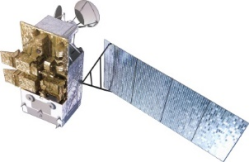
Figure 1. Physical image of FY-3D meteorological satellite.
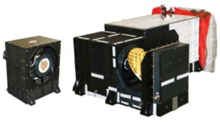
Figure 2. Physical image of MERSI.
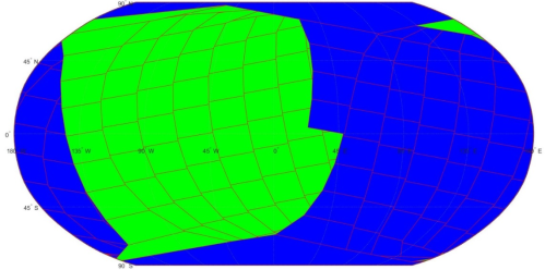
Figure 3. Coverage of MERSI-II data at 250 m resolution from Fengyun-3D Satellite.
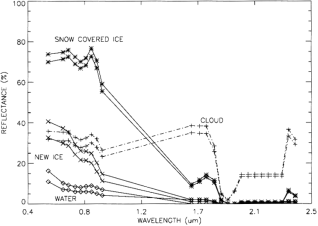
Figure 4. Reflectance curves for ice, clouds, and water in the Bering Sea region based on statistical analysis of MAS data for each band [19].
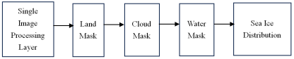
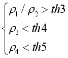
Figure 5. Sea ice identification model.
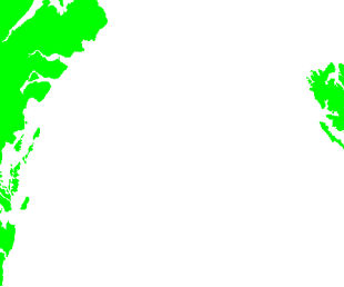
Figure 6.
Land mask (green = land, white = other).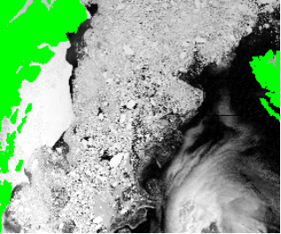
Figure 7. Result of applying the land mask.

Figure 8. Cloud mask image (red = cloud, white = other).
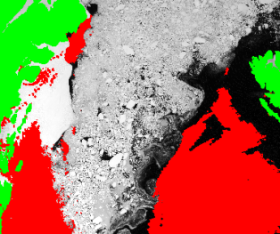
Figure 9. Result of applying the land and cloud masks.
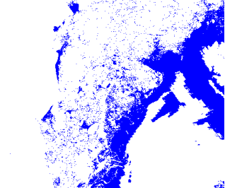
Figure 10. Seawater mask image (blue = seawater, white = other).
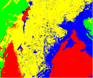
Figure 11. Ice identification results.
Information